Module 6: Proportional & Bivariate

 

     Proportional symbols are an excellent and interesting method for mapping bivariate data; however, they can be rather difficult to implement effectively. This is due to the way ArcGIS handles the symbols, the negative values must be separated into their own layer and made positive. These dual layers cause potential issues with larger symbols in one layer obscuring smaller symbols of the other layer. In the map above (top), this issue was alleviated by changing the layers' positions in the drawing order and by adjusting the transparency of the symbols. Although this was a viable solution for the above map (top), this may not be the case for every dataset and caution should be exercised when attempting to utilize this symbology.

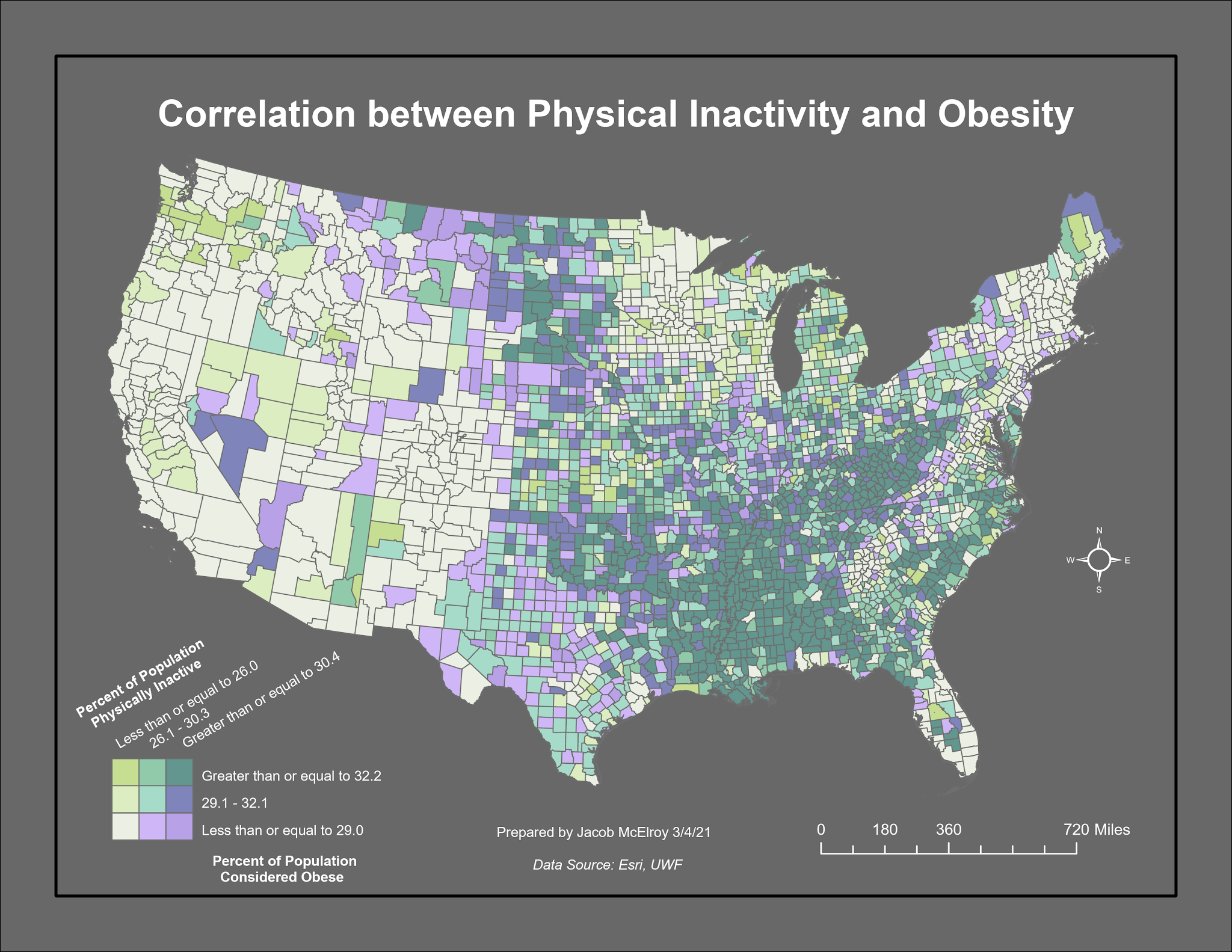
     The process of mapping bivariate data via choropleth is more complex than that of proportional symbols. New text fields are created in the layer's attribute table, one for each variable and a third for the combined final product. The three-class qauntile symbology and histogram are used for each variable to find the breakpoints for each class. The features are selected according to which class they fall into for the first variable. The new field for this variable is populated using these selected classes, with each class being assigned a letter A-C. The same steps are taken for the second variable with the new field containing values of 1-3 rather than A-C. The final new field is populated by combining the new variable fields so that the values are combinations of A-C and 1-3. This combined field is then used in tandem with a unique values symbology to create a bivariate choropleth as shown above (bottom).

Module 5: Analytics

 

     The lab for analytics required us to create an infographic utilizing public health information from County Health Rankings. I chose to display data showcasing the relationship between sleep deprivation and physical wellness. The typography of the map was kept simple and an Arial font was used with bold, regular, and italic styles being applied depending upon the text. The variables were displayed via choropleth maps in the center of the layout with multi-hue symbologies. These maps were placed atop a light purple rectangle sitting in amidst a dark grey background. These design choices were implemented to enhance figure-ground. The colors for the bar and pie graphs were chosen from the map symobologies so that the various elements could be distinguished from each other while still matching a common theme. These graphs and the scatterplot were arranged above and below the maps so that the graphs lie on opposite sides of the layout from the map they share their colors with. This was done to create visual contrast.

Module 4: Color & Choropleth

 

     The linear and adjusted progression color ramps (bottom and middle) consist of a single hue, while the ColorBrewer ramp (top) contains both purples and reds. This presents more available colors to choose from when selecting for intermediate classes and aids in differentiating between classes. The lightest class for the ColorBrewer ramp is drastically lighter than those of the linear and adjusted ramps, this results in a greater range of options for the intermediate classes and also assists with discerning between classes.

Module 3: Terrain Visualization

 

     This week's lesson concerned the various methods for visualizing terrain features. We specifically discussed hillshading, hypsometric tinting, and contours. The lab assignment for the week was to create a Land Cover map for Yellowstone National Park, provided above, with reasonable color symbology and supported by terrain visualization via a hillshade effect. I began by grouping the various successional stages of plants into a single category based on their species. These land cover types were then colored in various shades of green, blue, and brown to represent the plants, water, and bare earth they respectively represented. A multi-directional hillshade was created from a DEM and placed underneath the Land Cover layer. I chose the multi-directional hillshade due to the increased level of terrain detail it displays compared to a traditional hillshade. The transparency for the Land Cover layer was set to 37 percent so that the terrain features depicted by the hillshade effect would be easily visible without fading the Land Cover layer to the point of being unreconizable. The colors for the Land Cover symbology were adjusted so that they remained distinct and intuitive to the data displayed but were not jarring nor competing for dominance in the visual hierarchy.

     I have constantly been frustrated with the appearance and perceived quality of hillshade effects that I have utilized, as they always appear somewhat blurred. The multi-directional hillshade alleviates this concern due to its increased level of detail. I am elated to have learned this technique and look forward to implementing it in future products.

Module 2: Coordinate Systems

 

       The lesson for our second week of class centered on coordinate systems. We explored various projected coordinate systems and the reasons for their respective application. Part of our assignment was to select a state of interest within the United States and create a map of that state utilizing an appropriate coordinate system of our own designation. I chose the state of Montana and implemented the NAD 1983 StatePlane Montana FIPS 2500 (Meters) coordinate system. I partially chose this system due to it being one of two coordinate systems commonly used within the United States, those being State Plane and Universal Transverse Mercator (UTM). The other reasons for selecting the State Plane system are that Montana has three UTM zones but only one State Plane zone. Due to the entirety of Montana being encompassed by this singular State Plane zone, the State Plane system can be considered reliably accurate for the entire state

Module 1: Map Design & Typography

     This week's lab focused on the 5 principles of cartographic design and the use of typography. We were tasked with creating several maps consistent with these design principles and utilizing various forms of typography and labels. The above image depicts one of the resulting maps from this exercise. The above general purpose reference map of San Francisco, California utilizes various font sizes, types, colors, and effects to efficiently communicate the data contained. Large and important features (San Francisco, Marin Peninsula, San Francisco Bay, etc.) are labeled with large font to indicate their size and importance, while the smaller and less significant features (parks, neighborhoods, Lake Erced, etc.) utilize smaller font sizes for their labels. Color was used to intuitively indicate the type of feature the label represents, in addition to distinguishing the various labels from each other and their surroundings. To aid in the contrast between labels and surroundings, some of the labels in the map were given halo or shadow effects. Various fonts were used to differentiate hydrographic labels from those of other features.

     Upon first glance, this lab seemed mundane and simple. As the I worked through the exercises, I realized that the assignments were complex and challenging. This was a pleasant surprise, resulting in my introduction to several new methods for organizing and labeling my maps. I look forward to implementing several of them in future productions.

Module 4: Spatial & Spectral Enhancements and Band Indices

 

     This weeks lab explored various methods of image preprocessing and band indices. The lab required us to utilize both ArcGIS Pro and Erdas Imagine to identify features in images via the implementation of various band combinations. We also were introduced to the NDVI function of Erdas Imagine and the utility of histograms in both programs. Using the various techniques learned throughout the lab, we were given spectral criteria for three features and tasked with identifying and presenting them. The resulting maps and there band combinations are depicted in the layout above. The label under each map states the feature that map accentuates.